The Fourier Transform of the Complex Gaussian

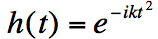
The Complex Gaussian

The complex Gaussian is a Gaussian Function with a imaginary argument. It is also can be viewed as a sinusoid with a phase that increases quadratically with time. This function arises in the study of optics. The function is given in Equation [1], where k is a positive real constant:

		[Equation 1]

To find the Fourier Transform of the Complex Gaussian, we will make use of the Fourier Transform of the Gaussian Function, along with the scaling property of the Fourier Transform.

To start, let's rewrite the complex Gaussian h(t) in terms of the ordinary Gaussian function g(t):

		[Equation 2]

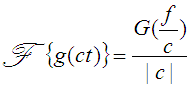
Now, we'd like to use the scaling property of the Fourier Transform directly, but note that the following equation only holds for c being real-valued (not a complex constant, as we are using in Equation [2]):

		[Equation 3]

The magnitude sign in Equation [3] arises because if c is real and negative, the integration limits will flip and the 1/c becomes -1/c (see Scaling Proof for Fourier Transforms. Hence, the generalization of Equation [3] to complex numbers is not valid.

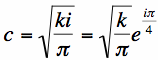
However, we are a little bit lucky in this case. The Gaussian Function of Equation [1] is well-defined when the argument becomes complex - that is, the complex exponential is well understood. This isn't the case in general - for instance, what is u(it) - the step function evaluated at a complex argument? There is no simple or consistent way to define it.

In this case, we have the constant c being given by:

		[Equation 4]

I apologize for the lack of rigor on this next statement, but basically we need the real and imaginary parts of the scaling constant c to be positive in order to avoid any additional minus signs that will show up in Equation [3]. This is because if the real and imaginary parts of c are positive, we won't need to do a sign change in the integration limits. Assuming k is positive, the resulting Fourier Transform follows since we know G(f), the Fourier Transform of the Gaussian already:

		[Equation 5]

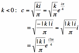
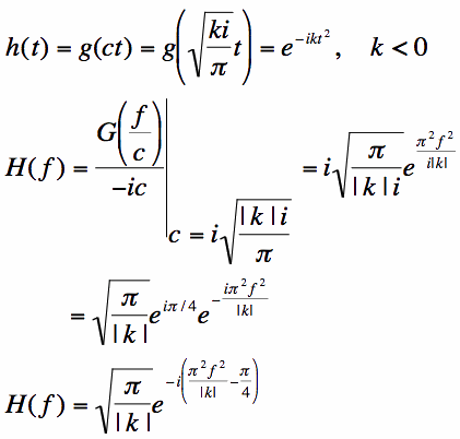
If on the other hand, k is negative, then the constant c in Equation [4] will will be given by:

		[Equation 6]

Hence, k has a negative real part and a positive imaginary part. By multiplying the constant c in Equation [6] by -i, we can force c to have a positive real and imaginary part. Hence, we can find the Fourier Transform of the complex Gaussian for the negative k case:

		[Equation 7]

Hence, the general solution for the Fourier Transform is:

		[Equation 8]

Note that if k=0, then the complex Gaussian is simply a constant, so the Fourier Transform will be the dirac-delta functional.