The Dirac-Delta Function - The Impulse
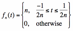
Consider the function, fn(t), shown described by equation [1], and plotted in Figure 1 for n=1 and n=5:
Figure 1. This is a square pulse with amplitude n and duration 1/n. (a)n=1 (b)n=5
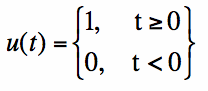
The unit step function is defined as:
The unit step is plotted in Figure 2:
Figure 2. The unit step function.
From equation [4], the dirac-delta can be thought of as being zero everywhere except where t=0, in which case it is infinite. This is
an acceptable viewpoint for the dirac-delta impulse function, but it is not very rigorous mathematically:
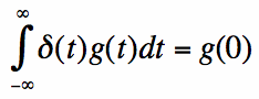
Probably the most useful property of the dirac-delta, and the most rigorous mathematical defintion is given in this section.
Consider any function g(t), that is continuous (and finite) at t=0. Then the following relationship always holds:
In [6], the integration region just needs to contain t=0, and doesn't necessarily need to go from -infinity to +infinity. This property
is extremely useful in signal processing, communication systems theory, quantum physics, etc. This is known as the 'sifting property' of
the impulse function. The more general version, assuming g(t) is continuous and finite at g(a) is:
This property is your friend whenever an integral is involved: it makes the integration extremely simple.
Finally, as a further note on notation, the impulse (shifted to the right by 1, given in equation [8])
is plotted as shown in Figure 3. It is graphed as a vertical arrow, since
it is zero everywhere, except where t=1, when it is more or less infinite.
Figure 3. The graph of the Dirac-Delta Impulse Function.
The Dirac-Delta function, also commonly known as the impulse function, is described on this page. This function (technically a functional) is one
of the most useful in all of applied mathematics.
To understand this function, we will several alternative definitions of the impulse function, in varying degrees of rigor. 1. Dirac-Delta: The Limit of a Sequence of Functions
 [1]
[1]
 [2]
[2]2. Dirac-Delta: The Derivative of the Step Function
 [3]
[3]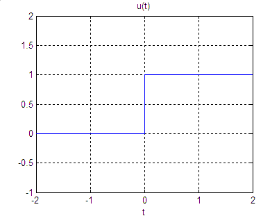
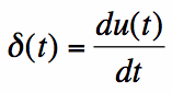 [4]
[4]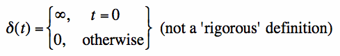 [5]
[5]3. Dirac-Delta: The Sifting Functional
 [6]
[6]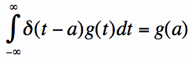 [7]
[7]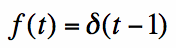 [8]
[8]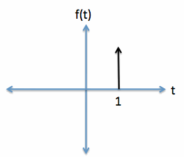
Previous: Intro to Complex Math
Fourier Transform Mathematical Topics
Fourier Transforms (Home)