Fourier Transform Applied to Partial Differential Equations

On the previous page on the Fourier Transform applied to differential equations, we looked at the solution to ordinary differential equations. On this page, we'll examine using the Fourier Transform to solve partial differential equations (known as PDEs), which are essentially multi-variable functions within differential equations of two or more variables. As an example of solving Partial Differential Equations, we will take a look at the classic problem of heat flow on an infinite rod. That is, essentially we are interested in the temperature of the rod; we'll call the temperature as a function of position (x) and time (t) by G(x, t). Side Note: solving heat flow on a circular ring is actually the original motivation for Fourier Series and Fourier Transforms by Fourier! 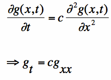Now, heat flow on a rod is governed by the partial differential equation: [Equation 1] A couple of things to note in equation [1]: The operator represents the partial derivative with respect to time. That is, the derivative is taken with respect to t while treating x as a constant. The same goes for the partial derivative with respect to x (t is held constant). To simplify, we will use the subscript notation for partial derivatives, as in the second line of Equation [1]. That is, g_x represents the partial derivative of g with respect to x The constant c is a positive number and is a measure of how quickly the heat diffuses from one part of the rod to another. We will introduce an initial condition and look to solve for the heat function g(x,t) for all values of t>0. That is, suppose we know the temperature distribution on the rod for all x at t=0: [Equation 2] We call the intial temperature distribution h(x). Our goal now is to solve the PDE in Equation [1] subject to the condition in Equation [2]. To accomplish this, we will use (you guessed it) the Fourier Transform. To start, let's take the Fourier Transform of Equation [1] with respect to x. 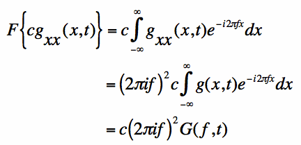That is, we will assume x is the variable and hold t constant. First, we will take the Fourier Transform of the right hand side of Equation [1]: [Equation 3] Note that in Equation [3], we are more or less treating t as a constant. The Fourier Transform is over the x-dependence of the function. We also define G(f,t) as the Fourier Transform with respect to x of g(x,t). 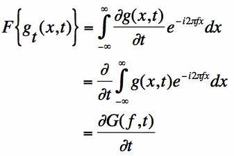The next step is to take the Fourier Transform (again, with respect to x) of the left hand side of equation [1]. To do this, we'll make use of the linearity of the derivative and integration operators (which enables us to exchange their order): [Equation 4] Now that we have the full Fourier Transform of Equation [1], we set Equation [3] equal to Equation [4]: [Equation 5] Equation [5] represents a simple Ordinary Differential Equation in the variable t; the function we seek is G(f,t). Using elementary differential equation methods, we obtain: [Equation 6] The function G(f, 0) represents the initial condition for the differential Equation in [5]. We also know that G(f, 0) is just the Fourier Transform with respect to x of g(x, 0); and from Equation [2] we know that g(x, 0) is just h(x). Hence, we re-write the initial condition as the Fourier Transform of h(x), and call it H(f): [Equation 7] Recall that the goal here is to get g(x, t). We can obtain this by taking the inverse Fourier Transform (with respect to x) of Equation [7]. Also, note that Equation [7] represents the product of two functions: H(f) and the Gaussian Function. As a result, hopefully you recognize that a convolution will be coming in the x domain. 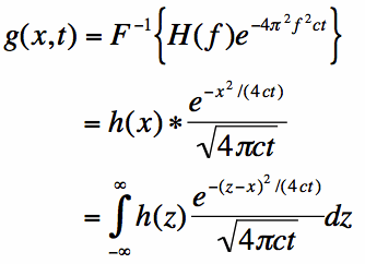Before that, we will take the inverse Fourier Transform of the Gaussian in Equation [7] (if you want to see how this is derived, see here): [Equation 8] Equation [8] can be used to take the inverse Fourier Transform of Equation [7]: [Equation 9] The result in Equation [9] represents the general solution of Equation [1], subject to the condition of Equation [2]. The result, in essence, represents how the initial heat distribution smooths itself out over time. That is, as t approaches 0, g(x,t) approaches h(x). This is because the Gaussian function becomes very sharp and approximates an impulse function. As time increases, the integration of Equation [9] represents a "smoothing out" or averaging of the initial temperature distribution h(x). This equation dictates precisely how heat spreads out on a rod.